Skip to content

Posts from the ‘Ecology’ Category

Chalk talk: How to model air temperature variation with height

In his latest chalk talk, Dr. Colin Campbell, environmental scientist at METER Group, teaches how to model vertical variation in temperature and how to estimate sensible heat flux.

Video transcript

Hello, everyone. My name is Dr. Colin Campbell, and I’m a senior research scientist here at METER Group. For today’s chalk talk, we’ll be talking about modeling vertical variation in temperature. In Figure 1, I’ve put together a graph that shows the maximum and minimum temperature with height and depth in the soil at some snapshot in time at a particular place. 

Figure 1. Maximum and minimum temperature with height and depth at a snapshot in time, in a particular place

It’s interesting to note that the change in temperature with depth in the soil is much faster than the change in temperature with height, whether we’re talking about a maximum or minimum. And the reason is that even though air is a good insulator, it also mixes really well. And that mixing is caused by eddies. And there’s a little more to that story. It depends specifically on surface heating by the sun through radiation and the cover type, whether it’s plants, rocks, boulders, straight soil, snow, or wind.

Equation 1

If we were going to model that, we would start by writing an equation (Equation 1) where a temperature at sun height, Z, above the surface (see variables noted in Figure 1), is equal to an aerodynamic surface temperature, T0, minus the sensible heat flux, divided by 0.4 times rho, CP, which is the volume specific heat of the air, times a variable called u*, which is the friction velocity. We multiply all that by the logarithm of z, the height above the surface minus d, which is the zero plane displacement, divided by z h, which is a roughness parameter. You might notice up here in the list of variables, that the zero plane displacement is 0.6 times H. H is the canopy height in meters. The rough roughness parameter can be estimated as 0.02 times the canopy height or times H. Now we have an equation that will help us model temperature with height. 

However, often we don’t know things like H, our sensible heat flux, and u*, our friction velocity. One of the things that we notice about this equation is that it’s set up somewhat like a linear equation. As you know, an example of a linear equation is something like Equation 2.

Equation 2

Figure 1 isn’t written quite that way, but if we look closely at the example below (Equation 3), this value could be our b, and this value our m, and this value could be our x. And if we do that, we actually can get some use out of graphing temperature with height. 

Equation 3

So we went out one day and measured this with a METER Group set of environmental sensors set up at certain heights above the surface. Here we placed sensors at 0.2 m, 0.4 m, 0.8 m, and 1.6 m above the ground. 

Table 1

To visualize this, in Figure 2 we graphed height on the y axis and temperature on the x axis, similar to the graph in Figure 1.

Figure 2. Graph showing the relationship between height and temperature

We know from Equation 1 that the axes for temperature and height should be switched because temperature is the dependent variable, and height is the independent variable. So if we switch axes it would look like the graph in Figure 3.

Figure 3. Graph showing the relationship between height and temperature where temperature is the dependent variable and height is the independent variable.

Figure 3 is graphed with the independent variable on the x axis and height on the y axis. If we fit this curve with today’s calculators, it would be fairly easy to get a curve that would fit that. But since it’s a linear equation, we can take the temperature data from Table 1 and the In ((Z-d)/ZH) data from Table 1 and graph them together.

Figure 4. Relationship between temperature and In Z-d/zh

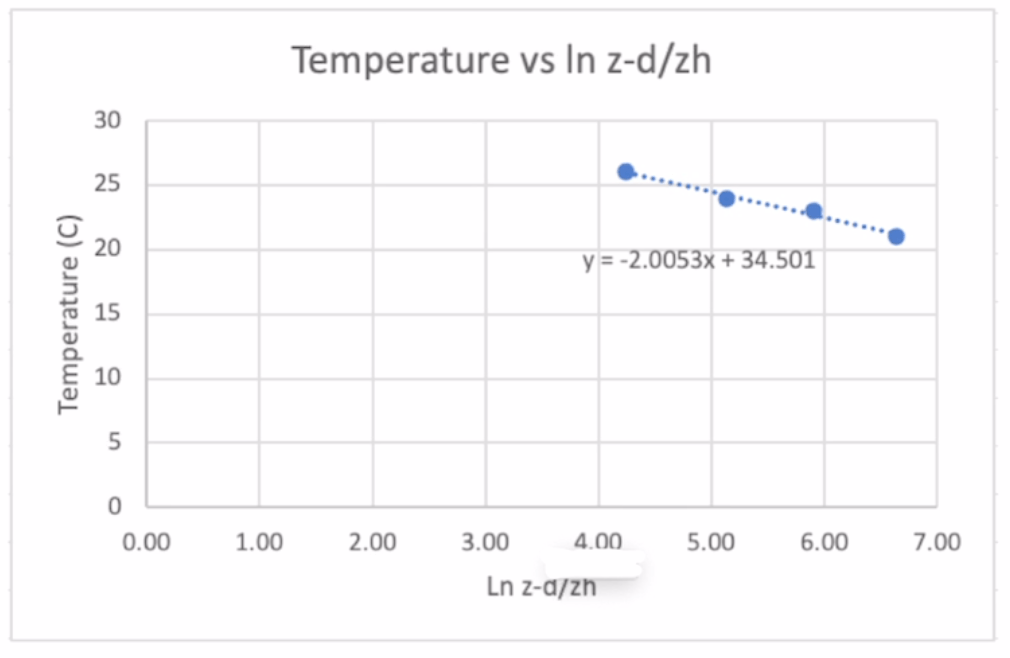
Figure 4 is a graph that shows what happens when we do that. Notice that, just like we suggested, it creates a linear equation (Equation 4). 

Equation 4

We learned in Figure 1 the B value was equal to t0 (our aerodynamic surface temperature). Since we know our surface temperature is 34.5 degrees, we can estimate what the temperature is down here at the surface, even though we only measured down 0.2 m. 

We also know from Equation 4 that our M value is equal to -2.01. And if we look at Equation 1, our slope value is below.

Equation 5 (the slope value from Equation 1)

So we can write

Equation 6

How to estimate sensible heat flux

Now, if we were interested in the sensible heat flux, which we often are, we can simply rearrange this equation to be

Equation 7

And in Figure 1, I forgot to give you this value, but for an air temperature of 20 degrees celsius, 

Equation 8

And then finally, a typical unit for friction velocity, which should be measured in the field over the specific canopy you are in, is about 0.2 meters per second.

Equation 9

So if we did this calculation, we would learned that there’s about 193 watts per meter squared of sensible heat flux coming off that surface. 

Equation 10

So if we can measure temperature at a few heights, we can estimate what the heat flux is coming off the surface assuming we know something about our canopy. Learn more about measuring and modeling environmental parameters at metergroup.com/environment. If you have any questions feel free to email Dr. Campbell at [email protected].

Learn more

Read about weather station best practices—>

Discover the ATMOS 41 All-In-One Weather Station—>

Download the Researcher’s complete guide to soil moisture—>

How to meet changing water demands in a growing population

In our latest podcast, Dr. Neil Hansen, BYU professor of environmental science, discusses water conservation, the latest research on getting more crop per drop, exciting applications of remote sensing, and the challenges we face trying to meet changing water demands in a growing population.

Listen now—>

Notes

Neil Hansen, PhD, is an environmental science professor at Brigham Young University. Learn more about Dr. Neil Hansen:

Neil’s curriculum vitae and publications

Subscribe:

https://www.metergroup.com/we-measure-the-world/

Follow us:

Disclaimer

The views and opinions expressed in the podcast and on this posting are those of the individual speakers or authors and do not necessarily reflect or represent the views and opinions held by METER.

Water Potential 101: What It Is. Why You Need It. How To Use It.

Soil is no longer a black box 

Advances in sensor technology and software now make it easy to understand what’s happening in your soil, but don’t get stuck thinking that only measuring soil water content will tell you what you need to know.

Water content is only one side of a critical two-sided coin. To understand when to water, plant-water stress, or how to characterize drought, you also need to measure water potential. 

Better data. Better answers.

Soil water potential is a crucial measurement for optimizing yield and stewarding the environment because it’s a direct indicator of the availability of water for biological processes. If you’re not measuring it, you’re likely getting the wrong answer to your soil moisture questions. Water potential can also help you predict if soil water will move, and where it’s going to go. Join METER soil physicist, Dr. Doug Cobos, as he teaches the basics of this critical measurement. Learn:

  • What is water potential?
  • Why water potential isn’t as confusing as it’s made out to be
  • Common misconceptions about soil water content and water potential
  • Why water potential is important to you

Register now—>

Presenter

Dr. Cobos is a Research Scientist and the Director of Research and Development at METER.  He also holds an adjunct appointment in the Department of Crop and Soil Sciences at Washington State University where he co-teaches Environmental Biophysics.  Doug’s Masters Degree from Texas A&M and Ph.D. from the University of Minnesota focused on field-scale fluxes of CO2 and mercury, respectively.  Doug was hired at METER to be the Lead Engineer in charge of designing the Thermal and Electrical Conductivity Probe (TECP) that flew to Mars aboard NASA’s 2008 Phoenix Scout Lander.  His current research is centered on instrumentation development for soil and plant sciences.

Episode 9: Pioneers of Environmental Measurement

What was the life of a scientist like before modern measurement techniques? In our latest podcast, Campbell Scientific’s Ed Swiatek and METER’s Dr. Gaylon Campbell discuss their association with three pioneers of environmental measurement.

Learn what it was like to practice science on the cutting edge. Discover the creative lengths they went to and what crazy things they cobbled together to get the measurements they needed.

Listen now—>

Ranching, Wildfires, & Global Sustainability

Check out our latest podcast, where Dr. Richard Gill discusses his global research projects including climate change on the Wasatch Plateau, ranch sustainability in Colorado, reef studies in Samoa, and wildfires in the Mojave Desert.

Landscape in Samoa

He focuses on the connection between the ecology of a place and the communities of people that inhabit it, and how scientists can protect socially and ecologically vulnerable populations by collaborating equally with them. Unless they’re sharks. He found out they’re typically not open to collaboration.

Listen now—>

Learn more about Dr. Gill

Richard Gill, PhD, is an ecologist and department chair in biology at Brigham Young University.

Links to learn more about Dr. Richard Gill:

Richard’s biography

Richard’s ResearchGate

Subscribe:

https://www.metergroup.com/we-measure-the-world/

Follow us:

https://twitter.com/meter_env

https://www.linkedin.com/showcase/meterenvironment/

Ticking Time Bomb: Climate Change In Antarctica

Dr. Marco Bittelli, soil physics wizard and pretty much the most interesting guy we know, discusses his exciting research projects in Italy and Antarctica. Plus, he shares insights on cutting-edge measurement methods, climate change, jazz guitar music, and more.

Marco Bittelli, PhD, is an associate professor in the Department of Agricultural and Food Science at the University of Bologna in Italy.

Listen now—>

Links to learn more about Dr. Marco Bittelli

Marco’s ResearchGate

Marco’s publications

Subscribe: https://www.metergroup.com/we-measure-the-world/

Follow us: https://twitter.com/meter_env

Hydraulic Conductivity: How Many Measurements Do You Need?

Two researchers show easier methods conform to standards

If you’re measuring saturated hydraulic conductivity with a double ring infiltrometer, you’re lucky if you can get two tests done in a day. For most inspectors, researchers, and geotechs—that’s just not feasible. Historically, double ring methods were the standard, however the industry is now more accepting of faster single ring methods with the caveat that enough locations are tested. But how many locations are enough?

Triple the tests you run in a day

Drs. Andrea Welker and Kristin Sample-Lord, researchers at Villanova University, are changing the way infiltration measurements are captured while keeping the standards of measurement high. They ran many infiltration tests with three types of infiltrometers with a variety of sizes and soil types. In this 30-minute webinar, they’ll discuss what they found to be the acceptable statistical mean for a single rain garden. Plus, they’ll reveal the pros and cons of each infiltrometer type and which ones were the most practical to use. Learn:

  • What types of sites were tested
  • How the spot measurements compared with infiltration rates over the whole rain garden
  • Pros and cons of each infiltrometer and how they compared for practicality and ease of use
  • What is an acceptable number of measurements for an accurate assessment

Register now—>

Presenters

Dr. Andrea Welker, PE, F.ASCE, ENV SP, is a Professor of Civil and Environmental Engineering and the Associate Dean for Academic Affairs at Villanova University. She joined Villanova after obtaining her PhD at the University of Texas at Austin. Her research focuses on the geotechnical aspects of stormwater control measures (SCMs) and the effectiveness of SCMs at the site and watershed scale.

Dr. Kristin Sample-Lord, P.E., is an Assistant Professor of geotechnical and geoenvironmental engineering in the Civil and Environmental Engineering Department at Villanova University. She received her PhD and MS from Colorado State University. Her research includes measurement of flow and transport in soils, with specific focus on green infrastructure and hydraulic containment barriers.

Related article: How to measure soil hydraulic conductivity
Related article: Which grain size analysis method is right for you?

Improve Your Plant Study: 3 Types of Environmental Data You May Be Missing

What data are you missing?

The environment plays a large role in any plant study. Ensuring you’re capturing weather and other environmental parameters in the best way allows you to draw better conclusions. To accurately assess plant stress tolerance, you must first characterize all environmental stressors. And you can’t do that if you’re only looking at above-ground weather data.

For example, drought studies are notoriously difficult to replicate and quantify. Knowing what kind of soil moisture data to capture can help you quantify drought, allowing you to accurately compare data from different years and sites.

Get better, more accurate conclusions

It’s important for your environmental data to accurately represent the environment of your site. That means not only capturing the right parameters but choosing the right tools to capture them. In this 30-minute webinar, application expert Holly Lane discusses how to improve your current data and what data you may not be collecting that will optimize and improve the quality of your plant study. Find out:

  • How to know if you’re asking the right questions
  • Are you using the right atmospheric measurements? And are you measuring weather in the right location?
  • Which type of soil moisture data is right for the goals of your research or variety trial
  • How to improve your drought study, why precipitation data is not enough, and why you don’t need to be a soil scientist to leverage soil data
  • How to use soil water potential
  • How accurate your equipment should be for good estimates
  • Key concepts to keep in mind when designing a plant study in the field
  • What ancillary data you should be collecting to achieve your goals

Register now—>

Presenter

Holly Lane has a BS in agricultural biotechnology from Washington State University and an MS in plant breeding from Texas A&M, where she focused on phenomics work in maize. She has a broad range of experience with both fundamental and applied research in agriculture and worked in both the public and private sectors on sustainability and science advocacy projects. Through the tri-societies, she advocated for agricultural research funding in DC. Currently, Holly is an application expert and inside sales consultant with METER Environment.

Evapotranspiration: Pitfalls to Avoid and Why It’s Easier Than You Think

Mistakes that kill your estimates

Measuring evapotranspiration (ET) to understand water loss from a native or a managed ecosystem is easier than it looks, but you have to know what you’re doing.

Learn causes and implications of uncertainty

If you can’t spend the time or money on a full eddy-covariance system, you’ll have to be satisfied with making some assumptions using equations such as Penman-Monteith.

Like any model, the accuracy of the output depends on the quality of the inputs, but do you know what measurements are critical for success? Plus, as your instrumentation gets more inaccurate, the errors get larger. If you’re not careful, you can end up with no idea what’s happening to the water in your system.

Get the right number every time

You don’t have to be a meteorologist or need incredibly expensive equipment to measure ET effectively. In this 30-minute webinar, Campbell Scientific application scientist Dr. Dirk Baker and METER research scientist Dr. Colin Campbell team up to explain:

  • The fundamentals of energy balance modeling to get ET
  • Assumptions that can simplify sensor requirements
  • What you must measure to get adequate ET estimates
  • Assumptions and common pitfalls
  • How accurate your equipment should be for good estimates
  • Causes and implications of uncertainty

WATCH IT NOW—>

Presenters

Dr. Dirk V. Baker has been with Campbell Scientific since 2011 and is an Application Research Scientist in the Environmental Group. Areas of interest include ecology, agriculture, and meteorology—among others. He has a bachelor’s degree in wildlife biology and a doctorate in weed science, both from Colorado State University. Dirk’s graduate and postdoctoral research centered around measuring and modeling wind-driven plant dispersal.

Dr. Colin Campbell has been a research scientist at METER for 20 years following his Ph.D. at Texas A&M University in Soil Physics. He is currently serving as Vice President of METER Environment. He is also adjunct faculty with the Dept. of Crop and Soil Sciences at Washington State University where he co-teaches Environmental Biophysics, a class he took over from his father, Gaylon, nearly 20 years ago. Dr. Campbell’s early research focused on field-scale measurements of CO2 and water vapor flux but has shifted toward moisture and heat flow instrumentation for the soil-plant-atmosphere continuum.

Learn more

Download the “Complete guide to irrigation management”—>

Soil Electrical Conductivity: Managing Salts for Sustained High Yields

Managing salts: Why you should care more

Mismanagement of salt applied during irrigation ultimately reduces production—drastically in many cases. Irrigating incorrectly also increases water cost and the energy used to apply it.

Understanding the salt balance in the soil and knowing the leaching fraction, or the amount of extra irrigation water that must be applied to maintain acceptable root zone salinity is critical to every irrigation manager’s success. Yet monitoring soil salinity is often poorly understood.

Measure EC for consistently high crop yields

In this webinar, world-renowned soil physicist Dr. Gaylon Campbell teaches the fundamentals of measuring soil electrical conductivity (EC) and how to use a tool that few people think about—but is absolutely essential for maintaining crop yield and profit. Learn:

  • The sources of salt in irrigated agriculture
  • How and why salt affects plants
  • How salt in soil is measured
  • How common measurements are related to the amount of salt in soil
  • How salt affects various plant species
  • How to perform the calculations needed to know how much water to apply for a given water quality

Register now—>

Presenter

Dr. Gaylon S. Campbell has been a research scientist and engineer at METER for over 20 years, following nearly 30 years on faculty at Washington State University. Dr. Campbell’s first experience with environmental measurement came in the lab of Sterling Taylor at Utah State University making water potential measurements to understand plant water status.

Dr. Campbell is one of the world’s foremost authorities on physical measurements in the soil-plant-atmosphere continuum. His book written with Dr. John Norman on Environmental Biophysics provides a critical foundation for anyone interested in understanding the physics of the natural world. Dr. Campbell has written three books, over 100 refereed journal articles and book chapters, and has several patents.

Learn more

Download the “Complete guide to irrigation management”—>