In our latest podcast, Dr. Cristine Morgan, one of the US’s premier soil scientists and Chief Scientific Officer at the Soil Health Institute shares her views on soil health: what it is, how to quantify it, what’s the payoff, and why it’s so critical to our success as a society.
“Our soils support 95 percent of all food production, and by 2060, our soils will be asked to give us as much food as we have consumed in the last 500 years.” (Credit: https://livingsoilfilm.com/)
Her thoughts? “We all live or die by soil, literally. We just have to remind people that it’s about quality of life. It’s about the food that you eat. It’s about the safety and welfare of your children.”
Dr. Cristine Morgan is the Chief Scientific Officer at the Soil Health Institute in North Carolina. Learn more about the Soil Health Institute on their website.
The views and opinions expressed in the podcast and on this posting are those of the individual speakers or authors and do not necessarily reflect or represent the views and opinions held by METER.
In our latest podcast episode, Kevin Hyde, manager of the Montana Mesonet, discusses his views on predicting and mitigating the effects of flood and drought.
Montana’s large geographical area makes mesonet equipment maintenance a challenge.
He also shares how to build a robust weather network with high-quality data on a small budget, why setups should include other measurements such as soil moisture and NDVI, and the genius way he handles maintenance over such a large geographical area.
The views and opinions expressed in the podcast and on this posting are those of the individual speakers or authors and do not necessarily reflect or represent the views and opinions held by METER.
In his latest chalk talk, Dr. Colin Campbell, environmental scientist at METER Group, teaches how to model vertical variation in temperature and how to estimate sensible heat flux.
Video transcript
Hello, everyone. My name is Dr. Colin Campbell, and I’m a senior research scientist here at METER Group. For today’s chalk talk, we’ll be talking about modeling vertical variation in temperature. In Figure 1, I’ve put together a graph that shows the maximum and minimum temperature with height and depth in the soil at some snapshot in time at a particular place.
Figure 1. Maximum and minimum temperature with height and depth at a snapshot in time, in a particular place
It’s interesting to note that the change in temperature with depth in the soil is much faster than the change in temperature with height, whether we’re talking about a maximum or minimum. And the reason is that even though air is a good insulator, it also mixes really well. And that mixing is caused by eddies. And there’s a little more to that story. It depends specifically on surface heating by the sun through radiation and the cover type, whether it’s plants, rocks, boulders, straight soil, snow, or wind.
Equation 1
If we were going to model that, we would start by writing an equation (Equation 1) where a temperature at sun height, Z, above the surface (see variables noted in Figure 1), is equal to an aerodynamic surface temperature, T0, minus the sensible heat flux, divided by 0.4 times rho, CP, which is the volume specific heat of the air, times a variable called u*, which is the friction velocity. We multiply all that by the logarithm of z, the height above the surface minus d, which is the zero plane displacement, divided by z h, which is a roughness parameter. You might notice up here in the list of variables, that the zero plane displacement is 0.6 times H. H is the canopy height in meters. The rough roughness parameter can be estimated as 0.02 times the canopy height or times H. Now we have an equation that will help us model temperature with height.
However, often we don’t know things like H, our sensible heat flux, and u*, our friction velocity. One of the things that we notice about this equation is that it’s set up somewhat like a linear equation. As you know, an example of a linear equation is something like Equation 2.
Equation 2
Figure 1 isn’t written quite that way, but if we look closely at the example below (Equation 3), this value could be our b, and this value our m, and this value could be our x. And if we do that, we actually can get some use out of graphing temperature with height.
Equation 3
So we went out one day and measured this with a METER Group set of environmental sensors set up at certain heights above the surface. Here we placed sensors at 0.2 m, 0.4 m, 0.8 m, and 1.6 m above the ground.
Table 1
To visualize this, in Figure 2 we graphed height on the y axis and temperature on the x axis, similar to the graph in Figure 1.
Figure 2. Graph showing the relationship between height and temperature
We know from Equation 1 that the axes for temperature and height should be switched because temperature is the dependent variable, and height is the independent variable. So if we switch axes it would look like the graph in Figure 3.
Figure 3. Graph showing the relationship between height and temperature where temperature is the dependent variable and height is the independent variable.
Figure 3 is graphed with the independent variable on the x axis and height on the y axis. If we fit this curve with today’s calculators, it would be fairly easy to get a curve that would fit that. But since it’s a linear equation, we can take the temperature data from Table 1 and the In ((Z-d)/ZH) data from Table 1 and graph them together.
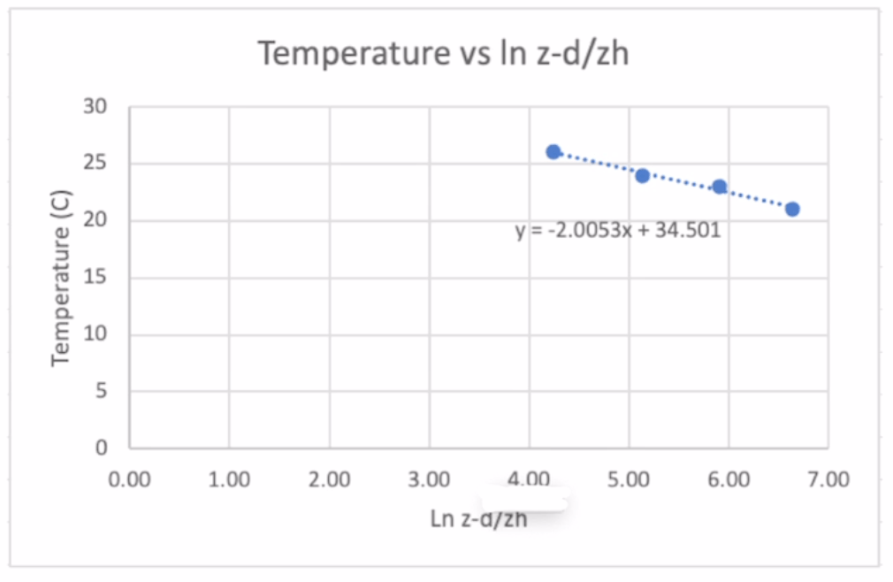
Figure 4. Relationship between temperature and In Z-d/zh
Figure 4 is a graph that shows what happens when we do that. Notice that, just like we suggested, it creates a linear equation (Equation 4).
Equation 4
We learned in Figure 1 the B value was equal to t0 (our aerodynamic surface temperature). Since we know our surface temperature is 34.5 degrees, we can estimate what the temperature is down here at the surface, even though we only measured down 0.2 m.
We also know from Equation 4 that our M value is equal to -2.01. And if we look at Equation 1, our slope value is below.
Equation 5 (the slope value from Equation 1)
So we can write
Equation 6
How to estimate sensible heat flux
Now, if we were interested in the sensible heat flux, which we often are, we can simply rearrange this equation to be
Equation 7
And in Figure 1, I forgot to give you this value, but for an air temperature of 20 degrees celsius,
Equation 8
And then finally, a typical unit for friction velocity, which should be measured in the field over the specific canopy you are in, is about 0.2 meters per second.
Equation 9
So if we did this calculation, we would learned that there’s about 193 watts per meter squared of sensible heat flux coming off that surface.
Equation 10
So if we can measure temperature at a few heights, we can estimate what the heat flux is coming off the surface assuming we know something about our canopy. Learn more about measuring and modeling environmental parameters at metergroup.com/environment. If you have any questions feel free to email Dr. Campbell at [email protected].
In our latest podcast, Dr. Neil Hansen, BYU professor of environmental science, discusses water conservation, the latest research on getting more crop per drop, exciting applications of remote sensing, and the challenges we face trying to meet changing water demands in a growing population.
The views and opinions expressed in the podcast and on this posting are those of the individual speakers or authors and do not necessarily reflect or represent the views and opinions held by METER.
Advances in sensor technology and software now make it easy to understand what’s happening in your soil, but don’t get stuck thinking that only measuring soil water content will tell you what you need to know.
Water content is only one side of a critical two-sided coin. To understand when to water, plant-water stress, or how to characterize drought, you also need to measure water potential.
Better data. Better answers.
Soil water potential is a crucial measurement for optimizing yield and stewarding the environment because it’s a direct indicator of the availability of water for biological processes. If you’re not measuring it, you’re likely getting the wrong answer to your soil moisture questions. Water potential can also help you predict if soil water will move, and where it’s going to go. Join METER soil physicist, Dr. Doug Cobos, as he teaches the basics of this critical measurement. Learn:
What is water potential?
Why water potential isn’t as confusing as it’s made out to be
Common misconceptions about soil water content and water potential
Dr. Cobos is a Research Scientist and the Director of Research and Development at METER. He also holds an adjunct appointment in the Department of Crop and Soil Sciences at Washington State University where he co-teaches Environmental Biophysics. Doug’s Masters Degree from Texas A&M and Ph.D. from the University of Minnesota focused on field-scale fluxes of CO2 and mercury, respectively. Doug was hired at METER to be the Lead Engineer in charge of designing the Thermal and Electrical Conductivity Probe (TECP) that flew to Mars aboard NASA’s 2008 Phoenix Scout Lander. His current research is centered on instrumentation development for soil and plant sciences.
What was the life of a scientist like before modern measurement techniques? In our latest podcast, Campbell Scientific’s Ed Swiatek and METER’s Dr. Gaylon Campbell discuss their association with three pioneers of environmental measurement.
Learn what it was like to practice science on the cutting edge. Discover the creative lengths they went to and what crazy things they cobbled together to get the measurements they needed.
Check out our latest podcast, where Dr. Richard Gill discusses his global research projects including climate change on the Wasatch Plateau, ranch sustainability in Colorado, reef studies in Samoa, and wildfires in the Mojave Desert.
Landscape in Samoa
He focuses on the connection between the ecology of a place and the communities of people that inhabit it, and how scientists can protect socially and ecologically vulnerable populations by collaborating equally with them. Unless they’re sharks. He found out they’re typically not open to collaboration.
Dr. Marco Bittelli, soil physics wizard and pretty much the most interesting guy we know, discusses his exciting research projects in Italy and Antarctica. Plus, he shares insights on cutting-edge measurement methods, climate change, jazz guitar music, and more.
Marco Bittelli, PhD, is an associate professor in the Department of Agricultural and Food Science at the University of Bologna in Italy.
In our latest We Measure the World podcast, we interview Oregon State University researcher Dalyn McCauley
about her experience developing a site-specific decision support tool for on-farm management of crop damaging weather events—and techniques she used to help the grower implement changes for quality and yield improvements.
When you irrigate in a greenhouse or growth chamber, you need to get the most out of your substrate so you can maximize the yield and quality of your product.
But if you’re lifting a pot to gauge how much water is in the substrate, it’s going to be difficult—if not impossible—to achieve your goals. To complicate matters, soil substrates and potting mixes are some of the most challenging media in which to get the water exactly right.
Without accurate measurements or the right measurements, you’ll be blind to what your plants are really experiencing. And that’s a problem, because irrigating incorrectly will reduce yield, derail the quality of your product, deprive the roots of oxygen, and increase the risk of disease.
Supercharge yield, quality—and profit
At METER, we’ve been measuring soil moisture for over 40 years. Join Dr. Gaylon Campbell, founder, soil physicist, and one of the world’s foremost authorities on soil, plant, and atmospheric measurements, for a series of irrigation webinars designed to help you correctly control your crop environment to achieve maximum results. In this 30-minute webinar, learn:
Why substrates hold water differently than normal soil
How the properties of different substrates and potting mixes compare
Why it’s difficult if not impossible to irrigate correctly without accurately measuring the amount of water in the substrate
The fundamentals of measuring soil moisture: specifically water content and electrical conductivity
How measuring soil moisture helps you get the most out of the substrate you choose, so you can improve your product
Easy tools you can use to measure soil water in a greenhouse or growth chamber to maximize yields and minimize inputs